AGV Drive Wheel Odometry Accuracy: Dual-Loop Encoders, Radial Runout Tolerances, and Floor Slippage Compensation
Compare AGV drive wheel odometry, dual-loop encoders, runout tolerances and slip compensation. Use worked examples and an RFQ checklist to plan your design.
AGV drive wheel odometry accuracy depends on what happens between the encoder and the floor. A high-resolution motor encoder can report smooth rotor motion while gearbox lost motion, polyurethane deformation and traction slip change the distance the vehicle actually travels. Increasing the encoder bit count alone cannot resolve those downstream errors.
Scope and review date: Global / English, November 10, 2026. This guide supports mobile robot systems integrators, drive engineers and OEM procurement teams selecting wheel feedback and acceptance tests. The differential-drive equations below apply to two independently driven wheels on a planar floor; steered, skid-steer and Mecanum vehicles require their own kinematic models. All numerical sizing examples are hypothetical calculations, not measured product results or supplier performance guarantees.
The practical sequence is to identify the dominant error, allocate a tolerable contribution, choose a sensor location, and validate the assembled vehicle. This separates three different purchasing questions: how finely the encoder resolves angle, how accurately it measures that angle, and how reliably wheel rotation represents floor travel.
For component selection, compare the AGV forklift steering drive wheel selector and heavy-duty AGV drive wheel catalog. For a project review, send your load, floor conditions and odometry error budget.
1. The Physics of Odometry Error: Systematic vs. Non-Systematic Decomposition
A differential-drive model integrates incremental wheel displacements over each sampling interval. Let r_R and r_L be effective rolling radii, ΔN_R and ΔN_L the decoded counts, N_cpr the counts per wheel revolution, and b_eff the effective track width between wheel contact centers:
Δs_R = 2 * π * r_R * (ΔN_R / N_cpr)
Δs_L = 2 * π * r_L * (ΔN_L / N_cpr)

Δs   = (Δs_R + Δs_L) / 2
Δθ   = (Δs_R - Δs_L) / b_eff

x_next = x + Δs * cos(θ + Δθ / 2)
y_next = y + Δs * sin(θ + Δθ / 2)
θ_next = θ + Δθ
This midpoint integration is an approximation for sufficiently small motion increments. It assumes the wheel displacement estimates represent rolling travel. Slip, uneven floors and timing errors break that assumption even if every encoder count is received correctly.
Borenstein and Feng's odometry paper distinguishes systematic calibration errors from disturbances such as slip and floor irregularities. Unequal rolling diameters can bend a nominal straight trajectory; an incorrect effective track width biases turns. These effects depend on the path and can partly cancel in a one-direction closed-loop test, so they should not be described as always accumulating monotonically.
An equal radius scale error on both wheels primarily biases distance. A left/right mismatch also creates heading error, which then produces lateral error on the following straight segment. The resulting deviation depends on travel distance and track width; a wheel diameter mismatch alone cannot establish a universal drift figure.
Payload and temperature can create repeatable radius changes under controlled conditions, while changing floor contact and traction introduce less repeatable errors. Treating everything as a single fixed correction factor can hide this distinction. Record the operating condition alongside every calibration parameter.
2. Mechanical Error Propagation: Backlash, Hub Eccentricity, and Elastomeric Deflection
2.1 Gearbox Backlash and Reversal Lost Motion
For an output-referred angular backlash, the corresponding tire-periphery arc length is:
lost_motion_mm = wheel_radius_mm * (backlash_arcmin / 60) * π / 180For a hypothetical 250 mm wheel, the radius is 125 mm. A specified 3 arcmin output backlash corresponds to approximately 0.109 mm of arc length; 12 arcmin corresponds to 0.436 mm. These are geometric estimates, not a prediction of net route error. Reversal direction, torque, preload, shaft compliance and controller behavior determine how much lost motion appears in a maneuver.
Ask whether the gearbox specification is input- or output-referred and how it was measured. Backlash under a light inspection load is different from torsional deflection at operating torque. A motor encoder cannot distinguish output take-up from useful wheel travel; output feedback can observe the hub response, provided its mounting is downstream of the relevant play.
2.2 Radial Runout (TIR) and Cyclic Radius Modulation
Total Indicated Runout is the difference between maximum and minimum indicator readings over a revolution about the specified datum. Hub eccentricity, tread form error, bearing clearance and installation can all contribute. There is no single acceptable TIR for every AGV.
For a simplified circular wheel with small eccentricity, a useful screening model is:
r(φ) ≈ R + (TIR / 2) * sin(φ + phase)Here TIR / 2 is the amplitude only for the assumed eccentricity pattern. A real tread can have several lobes or local defects, and its loaded rolling behavior can differ from its unloaded inspection trace. Log a full revolution where possible rather than accepting only a single maximum reading.
A proposed 0.05 mm TIR target implies a 0.025 mm radial amplitude in this simplified model. It does not imply 0.05 mm positioning accuracy. Compare left/right phase, loaded behavior and vehicle motion before tightening a drawing tolerance that may increase manufacturing cost without addressing the dominant error.
2.3 Polyurethane Deflection Under Variable Payload
Static axle height and dynamic rolling radius are different quantities. Shore hardness alone does not establish either value: compound formulation, tread thickness, speed, temperature, load history and wheel geometry also matter. Avoid assigning a universal percentage of radius loss or a universal conversion factor from static compression to rolling radius.
Measure effective rolling radius using independent ground travel over several complete revolutions on a controlled surface:
r_eff = reference_distance / (2 * π * wheel_revolutions)Repeat empty and laden, in both directions, after thermal stabilization. Use low acceleration to reduce slip during calibration, document the reference instrument uncertainty, and repeat the measurement to assess scatter. If the loaded and unloaded results differ beyond the distance error budget, maintain separate validated calibration values or a bounded load-dependent model.
3. Dual-Loop Encoder Architecture vs. Conventional Single Motor Feedback
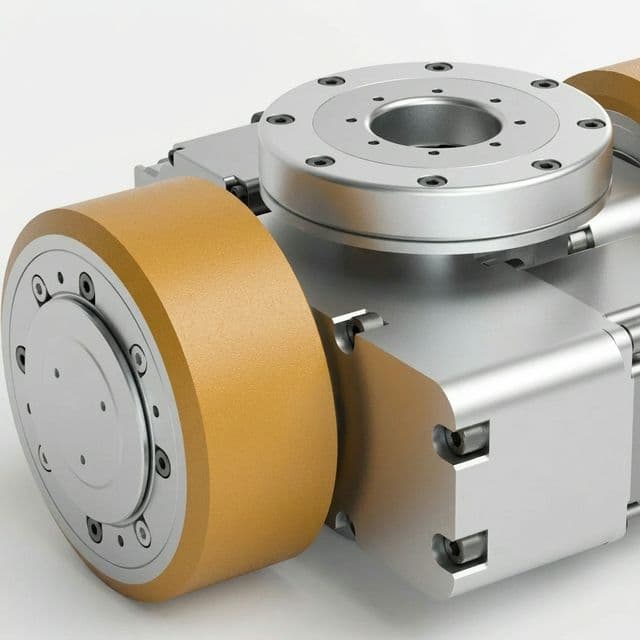
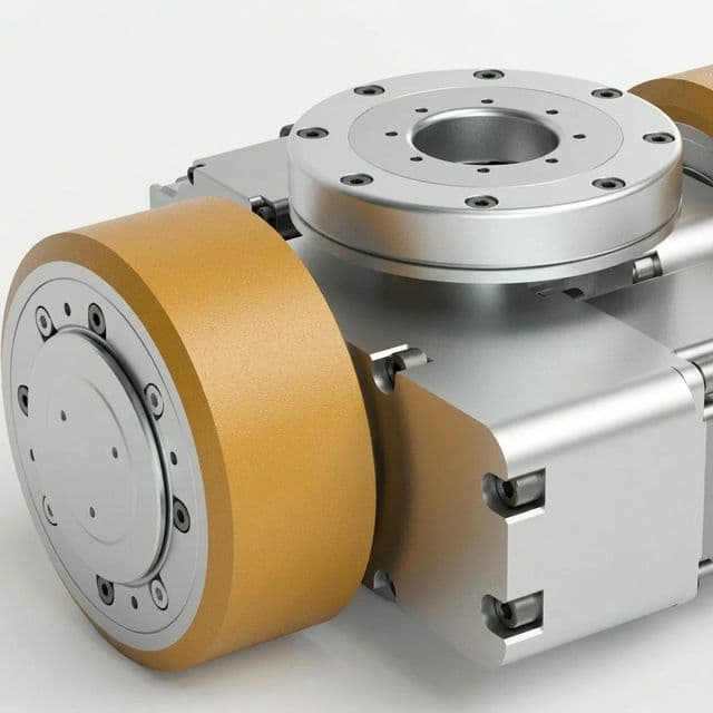
Assembly illustration only; the image does not establish encoder topology, measured runout or odometry performance.
A motor-side encoder supports commutation and motor control. An encoder on the wheel output can provide a separate observation of hub rotation. Using both observations for estimation is distinct from closing a dual-loop servo controller; the latter requires compatible hardware, filtering and stability tuning.
Motor encoder -> motor control
      |
Motor -> gearbox -> hub -> tread -> floor
                     |
               Output encoder -> hub-angle feedback / odometry

Unpowered tracking wheel -> separate travel estimate
Independent pose reference -> drift correction / validation
An output encoder observes the rotation after the gearbox. It does not remove the gearbox's physical backlash or torsional compliance, and it cannot observe slip between the tread and the floor. Loose mounting downstream of the sensor can remain invisible. Design the control bandwidth around measured dynamics rather than copying a generic loop frequency.
An unpowered measuring wheel avoids transmitting vehicle drive torque, which can make it less sensitive to drive-wheel spin. It still needs friction to overcome bearing drag and rotational inertia. Dust, liquid films, lateral scrub, contact loss and preload variation can introduce its own errors. Its signal is an incremental travel estimate, not an absolute ground-position reference.
Likewise, a multi-turn absolute encoder may recover shaft position after a power cycle if its design supports it. That does not recover the vehicle's global pose after wheel slip, lifting or unobserved motion. Verify recovery behavior explicitly in the vehicle commissioning procedure.
4. Encoder Topologies Compared: Motor-Mounted, Output-Axle, and Auxiliary Measuring Wheels
Select feedback by the error it can observe and the validation burden it creates:
| Feedback topology | Useful observation | Error that remains | Selection condition |
|---|---|---|---|
| Motor-mounted encoder | Rotor angle and motor velocity | Gearbox motion, radius variation and floor slip | Existing drivetrain error fits the vehicle budget |
| Direct-drive wheel encoder | Wheel rotation without a reduction gearbox | Tread deformation, eccentricity and floor slip | Motor torque and thermal packaging suit direct drive |
| Motor plus output-axle encoder | Hub response relative to motor rotation | Floor slip and motion downstream of output sensing | Measured reversal error justifies added feedback |
| One auxiliary measuring wheel | Travel component along its rolling direction | Own slip, bounce and lateral scrub; no full planar pose | Independent travel channel is useful and contact can be maintained |
| Two parallel measuring wheels | Travel and heading increments with known spacing | Shared floor disturbances and radius errors | Differential geometry and installation are validated |
| Two orthogonal measuring wheels | Two local displacement components | Rotation remains unobservable without another heading source | Holonomic motion needs independent heading and offset compensation |
| Wheel odometry plus external localization | Relative motion plus referenced pose corrections | Reference outages, sensor ambiguity and timing errors | Route and docking tests establish acceptable behavior during outages |
Sensor Technology and Electrical Interfaces
Optical, magnetic and inductive encoders all require model-specific comparison. Check specified angular accuracy, repeatability, cyclic error, sealing, temperature range, vibration rating and installation tolerances. Bit count alone cannot rank them. Magnetic field susceptibility and optical contamination resistance depend on the complete sensor and enclosure, so avoid claims of universal immunity or guaranteed IP performance based on sensing principle.
For incremental encoders, define whether PPR means cycles per channel and whether the receiver uses x1, x2 or x4 decoding. As an example, 2,048 cycles per revolution becomes 8,192 decoded counts with x4 decoding. Confirm that the supplier uses the same terminology before using the value in software.
For BiSS-C or SSI, confirm the actual device's frame length, status bits, error checking, clock range, cable limit and sample timing. For CANopen, confirm the encoder profile and object mapping; a drive profile is not automatically an encoder profile. For EtherCAT, verify cycle time and distributed-clock support where required. An ordinary protocol connection does not make a sensor or control path safety rated.
At maximum wheel speed, calculate both per-channel input frequency and decoded counter throughput. Check timestamp alignment with the IMU and localization data as well as nominal update rate. A high-resolution encoder with delayed or unevenly sampled data can make velocity estimation worse during rapid acceleration.
5. The Borenstein UMBmark Calibration Framework: Isolating Diameter and Track Errors
UMBmark uses clockwise and counter-clockwise square paths to help separate systematic diameter-ratio and effective-track errors. A one-direction test can hide compensating errors. A straight-line distance check is also needed to establish the common wheel-radius scale.
A practical commissioning sequence is:
- Inspect tire condition, mounting, alignment and encoder scaling before collecting data.
- Establish independent start and finish position and heading measurements. Keep localization corrections separate from the wheel-only estimate under test, while retaining the vehicle's protective functions.
- Select a square that fits the controlled test area. A 4 m side and five repeats per direction are an example test setup, not a requirement for every vehicle.
- Run both directions under consistent payload, speed and floor conditions. Record endpoint offsets, heading error and run-to-run spread.
- Fit diameter ratio and effective track width using a documented coordinate and sign convention. Follow the original method for correction equations rather than mixing formulas from different axis definitions.
- Validate the fitted parameters on separate runs and on an independent straight distance. Repeat at relevant loads to see whether a single parameter set remains adequate.
A smaller mean endpoint error shows improved systematic calibration; a large scatter still points to contact, slip, timing or reference-measurement issues. Report both quantities. UMBmark does not establish a universal percentage improvement, safety approval or millimeter docking guarantee, and its differential-drive correction model should not be copied directly to a steered forklift or Mecanum platform.
6. A Practical AGV Odometry Error Budget Matrix
The following matrix replaces a vehicle-class accuracy promise with measurable acceptance evidence. Allocate limits from your route and docking requirements before requesting hardware quotes. Contributions may be correlated, so adding every maximum or combining them by root-sum-square requires a justified model.
| Error contribution | How to estimate or measure it | Evidence to request | Acceptance boundary |
|---|---|---|---|
| Encoder quantization | Wheel circumference divided by counts per revolution | PPR/CPR definition and decoder settings | Resolution is finer than the allocated increment budget |
| Encoder angular accuracy | Convert specified angular error at wheel radius | Accuracy specification with installation conditions | Accuracy is checked separately from bit depth |
| Reversal lost motion | Output backlash arc length plus loaded reversal test | Gearbox test method and assembled response trace | Maneuver error fits the drivetrain allocation |
| Tread radial runout | Indicator trace about installed bearing datum | TIR report, datum and mounting conditions | Agreed manufacturing limit is met |
| Loaded rolling-radius change | Reference travel divided by revolutions at each load | Empty/laden calibration records | Residual distance bias fits the route budget |
| Left/right radius mismatch | Bidirectional trajectory calibration | Parameter values and independent validation runs | Heading and cross-track residuals are acceptable |
| Floor slip and contact loss | Compare wheel motion with independent reference | Representative floor and acceleration logs | Detection and degraded operation meet project criteria |
| Timing and sampling | Compare hardware timestamps and latency | Synchronization settings and dropout logs | Motion-dependent time error fits the estimate budget |
If the largest observed contribution is radius scale or slip, buying a finer encoder may offer little benefit. If reversal response dominates, compare output sensing with lower-backlash mechanics. This makes the RFQ a measurable engineering decision rather than a contest between encoder bit counts.
7. Floor Slippage Mitigation: Dynamic Traction Limits and Multi-Sensor Fusion
7.1 The Tractive Adhesion Boundary
For a simplified level-floor longitudinal model, let F_N_drive be the total normal force on driven wheels in newtons, m_total the total mass in kilograms, μ the available adhesion coefficient, and C_rr rolling resistance normalized to total vehicle weight:
a_limit ≈ μ * F_N_drive / m_total - C_rr * g

If F_N_drive = λ * m_total * g:
a_limit ≈ g * (μ * λ - C_rr)
This screening equation omits grade, trailer resistance, dynamic load transfer, turning forces and individual-wheel traction differences. Do not use a mass where a normal force in newtons is required. Measure floor/tread adhesion under representative contamination conditions instead of assigning a universal friction coefficient from hardness.
For a hypothetical case with μ = 0.25, driven load fraction λ = 0.60, C_rr = 0.02 and g = 9.81 m/s², the estimated acceleration limit is 9.81 * (0.25 * 0.60 - 0.02) = 1.275 m/s². A 1.5 m/s² command exceeds this simplified estimate and indicates a slip risk. It does not establish an approved acceleration limit or stopping distance.
7.2 Slip Detection and Estimator Weighting
Compare wheel-derived velocity or yaw rate with independent observations. An IMU comparison requires timestamp alignment, bias estimation, gravity compensation and accounting for sensor mounting location. Turning, ramps and vibration can create residuals without wheel slip; a single threshold cannot reliably distinguish them in every vehicle.
When independent evidence indicates wheel odometry is unreliable, reduce its estimator weight, bound acceleration or torque as appropriate, and follow the validated degraded-operation strategy. Set residual thresholds, persistence times and covariance changes from logs that include normal maneuvers and actual slip events. Avoid copying an arbitrary acceleration threshold or a fixed covariance multiplier into a production controller.
An auxiliary wheel can add a useful comparison channel, but two wheels on the same contaminated floor can fail together. Independent pose updates may limit drift when their environment supports reliable localization. Test reference outages and poor-feature routes as well as successful nominal operation.
8. Functional Safety and Safe Motion Monitoring
ISO 3691-4:2023 covers safety requirements and verification for driverless industrial trucks and their systems. IEC 61800-5-2:2016 addresses functional safety of safety-related power drive systems. These scopes help identify the relevant engineering documentation; public catalogue descriptions do not establish detailed compliance requirements for a particular vehicle.
Keep navigation estimation and safety validation distinct. Ordinary dual encoders, an EKF slip detector or a standard network interface do not by themselves establish a required safety integrity level. If feedback participates in protective-field selection or safe speed monitoring, obtain the applicable safety manual, architecture constraints, diagnostics, response times and validation evidence for the complete safety function.
Protective-field dimensions and stopping responses depend on measured stopping behavior, payload, floor conditions, sensing delays and the application risk assessment. This guide supplies no universal field length, encoder-disagreement threshold or stop category. Verify the applicable standard edition, including amendments, and market requirements when approving the project.
9. Step-by-Step OEM Procurement and Engineering RFQ Checklist
A useful RFQ states what must be demonstrated on the assembled system. Attach the error budget and request exceptions explicitly so supplier offers can be compared on the same basis.
- 1. Duty envelope: State gross mass, driven-wheel load range, center-of-gravity variation, speed, acceleration, grade and floor conditions.
- 2. Measurement requirement: Separate route drift, docking repeatability, absolute position accuracy and behavior during localization outages.
- 3. Tread runout: Define TIR limit, measurement surface, bearing datum, mounting torque, temperature and inspection procedure. Treat a proposed 0.05 mm limit as a project target requiring supplier confirmation.
- 4. Compound and load behavior: Request material identity, hardness tolerance, load-speed rating and rolling-radius characterization. Hardness alone cannot guarantee predictable deflection.
- 5. Drivetrain lost motion: Specify output-referred backlash, test torque, torsional stiffness and reversal-response evidence.
- 6. Sensor location: Mark motor, hub and auxiliary feedback locations on the drawing, including any play downstream of each sensor.
- 7. Encoder specification: State resolution, angular accuracy, interface, timing, count convention, maximum frequency and power-cycle behavior separately.
- 8. Environment and mounting: Specify required temperature, ingress, vibration, cable strain relief and electromagnetic compatibility for the actual installation.
- 9. Safety use: Identify whether feedback enters a safety function and request the relevant product safety documentation and integration limits.
- 10. Acceptance package: Agree inspection certificates, calibration records, representative loaded route tests, sample quantity, measurement uncertainty and rejection criteria.
Before freezing a specification, use the encoder wheel fit and signal pre-screen for its stated screening scope, then request a project-specific feedback review with your drawing and acceptance criteria. Screening results do not replace installed odometry tests.
10. Worked Engineering Sizing Example: 1,200 kg Autonomous Pallet Mover
Consider a hypothetical differential-drive pallet mover with 1,200 kg gross laden mass, 400 kg empty mass, two 200 mm nominal drive wheels, 600 mm track width and a 20:1 reduction. Assume the driven wheels share 60% of total weight equally. On level ground, each driven wheel carries approximately 1,177.2 N empty and 3,531.6 N laden. Actual load transfer must be checked separately.
Step 1: Calculate the Rolling-Radius Scale Error
Assume independent rolling tests have supplied effective radii of 99.81 mm empty and 99.42 mm laden. These are illustrative inputs, not compression-test data or predictions from Shore hardness.
If the controller stops when odometry reaches 30,000 mm using a fixed 100.00 mm radius, the idealized actual travel is:
actual_distance = commanded_odometry * r_actual / r_configured

Empty: 30,000 * 99.81 / 100.00 = 29,943 mm
Laden: 30,000 * 99.42 / 100.00 = 29,826 mm

Empty undershoot: 57 mm
Laden undershoot: 174 mm
Difference between conditions: 117 mm
This calculation assumes no slip, perfect heading and an odometry-distance stopping command. If instead a reference instrument measures an actual 30 m traverse, the estimation-error denominator changes to the actual radius. Always state which distance is held fixed.
Using a validated radius for each load condition can remove this scale bias in the ideal model. It cannot establish a residual error below 5 mm without measurement. Load cells may support model selection, while motor current alone is confounded by acceleration, grade and friction. Validate intermediate loads and temperature changes before interpolating.
Step 2: Calculate Reversal Lost Motion and Heading Sensitivity
Assume 10 arcmin output backlash. At a 100 mm wheel radius, the equivalent arc length is:
lost_motion = 100 * (10 / 60) * π / 180 = 0.291 mmIn a conservative maneuver scenario where the two wheel displacement errors have opposite signs, their differential contribution is approximately 0.582 mm. Dividing by the 600 mm track width gives 0.000970 rad, or about 0.0556°. If this heading error persists over a following 10 m straight segment, the lateral deviation is approximately 10,000 * sin(0.000970) = 9.7 mm.
This is a sensitivity calculation, not an inevitable docking failure. The actual sign, take-up, heading correction and fork clearances must be measured. An output encoder can make hub response observable, while final docking may still require an independent local reference.
Step 3: Check Resolution Against the Remaining Error Budget
An 18-bit axle encoder provides 262,144 positions per revolution. On a nominal 200 mm wheel, the corresponding circumference increment is π * 200 / 262,144 ≈ 0.00240 mm. This very fine quantization does not imply 0.00240 mm ground-position accuracy. Compare the encoder's specified angular accuracy, mounting error and floor-contact uncertainty before paying for more bits.
The purchasing conclusion for this example is conditional: characterize rolling radius first, evaluate reversal response second, and then choose enough encoder resolution and bandwidth to observe the remaining motion. Preserve the measurements and controller settings in the acceptance record so replacement wheels can be recalibrated consistently.
11. Frequently Asked Questions
Why can a 24-bit motor encoder still produce AGV odometry drift?
It measures rotor angle upstream of the gearbox. Backlash, coupling motion, changing rolling radius and floor slip remain downstream. More counts improve quantization but cannot establish ground displacement accuracy.
When should an OEM choose dual-loop encoders?
Choose output feedback when measured reversal error or compliance exceeds the allocated drivetrain error budget and the controller supports stable dual-feedback operation. An axle encoder observes output rotation; it does not measure tire slip or guarantee docking accuracy.
Does an auxiliary measuring wheel eliminate slip?
No. It avoids transmitting drive torque, which can reduce sensitivity to drive-wheel spin, but its own bearing drag, inertia, contamination, bounce and lateral scrub can still cause error. Validate contact preload and compare it with an independent reference.
What radial runout tolerance belongs on an AGV wheel drawing?
Derive the limit from the vehicle error budget and supplier capability. State the tread measurement surface, bearing datum, mounting torque, temperature and inspection method. A proposed 0.05 mm TIR limit is a project target to validate, not a universal AGV requirement.
How should payload-dependent rolling radius be calibrated?
Measure independent ground travel and wheel revolutions at representative loads, speeds and temperatures. Calculate effective radius as distance divided by two pi times revolutions. Static tire compression alone cannot establish the dynamic rolling radius.
When should UMBmark calibration be repeated?
Calibrate at commissioning and after wheel, gearbox, alignment or kinematic parameter changes. Set the ongoing interval from measured wear and drift. Use clockwise and counter-clockwise trials, and keep external localization corrections separate from the odometry estimate under test.
12. References and Source Boundaries
- Borenstein, J. and Feng, L. (1996): Measurement and Correction of Systematic Odometry Errors in Mobile Robots, IEEE Transactions on Robotics and Automation, 12(6). Supports systematic-error classification and bidirectional calibration. The university-hosted PDF returned HTTP 403 to automated retrieval during this review; it was not re-read, and no detailed correction formula or performance percentage is asserted here.
- ISO: ISO 3691-4:2023 — Driverless industrial trucks and their systems. Official catalogue scope checked November 10, 2026. Cited for the standard's scope, not a clause-level safety prescription or an odometry tolerance.
- IEC: IEC 61800-5-2:2016 — Safety requirements — Functional. Official catalogue scope checked November 10, 2026. The catalogue also identifies a consolidated version with Amendment 1:2026; confirm the applicable edition during procurement. No complete paid standard text was reviewed.
The worked arithmetic and RFQ framework are engineering screening guidance. They do not constitute physical test results, a customer case study or evidence that a particular product meets the example values.
13. Specify Your AGV Drive Wheel and Feedback Requirements
Prepare your maximum and minimum wheel loads, floor conditions, speed profile, proposed encoder location, runout drawing and acceptance budget before requesting a quote. Ask the supplier to identify which values are standard, which require customization and which remain subject to installed testing.
Explore AGV forklift steering drive wheels, compare heavy-duty drive assemblies, or send an engineering RFQ with your odometry requirements.